Current Balance: $29,842.77
Once you’ve set your goal, i.e. targeted date, to pay off your school loans. how do you determine how much to pay off each week, month or year depending on your preference in payment? You create an amortization schedule in excel and have some fun.
The first step is creating your based amortization schedule with either the default repayment schedule or your preferred repayment schedule. So let’s get started. For this example I’m going to calculate three difference loans with differing balances and interest rates with a standard repayment schedule of ten (10) years or 120 months.
Loan Amount Interest Rate
Loan 1 $24,500 6.8%
Loan 2 $12,200 3.5%
Loan 3 $ 5,000 5.0%
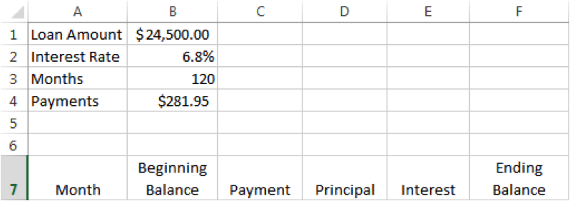
Insert your loan information into Excel which should look something like this:


Next, we want to calculate your payment by entering in an excel formula into the Payments cell. You may already have this information from your loan service provider, but this formula will also do the trick:
=ROUND(PMT($B$2/12,$B$3,-$B$1,0,2)
*TIP: The “B” cell will need to be changed to correspond with the appropriate loan, i.e. $G$2 and $L$2
Your spreadsheet should look something like this:

For the example, graduating with $41,700 in student loans results in a monthly payment of $455.62 under the standard payment plan. If this is too much, you can always modify the number of payments to equal the number in an extended payment plan. An extended payment plan would lower the monthly payment to $260.36. I chose this payment plan so I could have lower monthly payment and focus on paying off my highest interest loan.

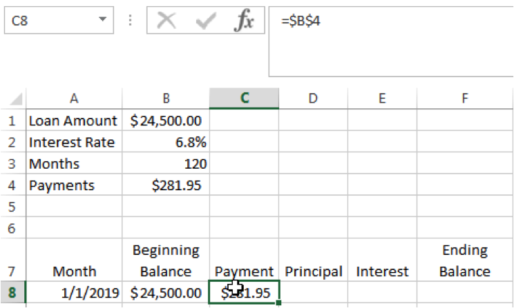
Next, we want to create the amortization schedule columns. The first step is to type out the following headers:

Then, we are going to start inserting the corresponding amounts and formulas:
1. Under “Month” enter in your first payment due date.
2. Under “Beginning Balance” enter in the loan amount from B1
3. Under “Payment” enter in payment in B4 as a stationary cell: Type “=$B$4”

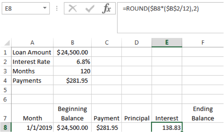
4. Under “Interest” enter in the following formula: =ROUND($B8*($B$2/12),2)

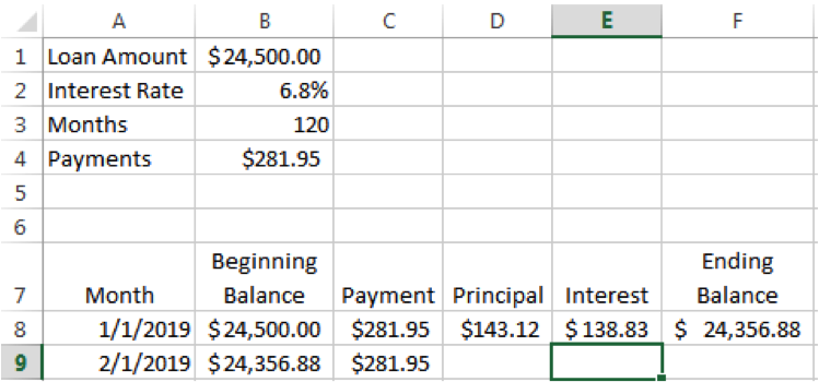
5. Under “Principal” enter in the following formula: =C8-E8 This subtracts the interest you paid from the payment amount, which lets you know what you’ve paid towards your principal balance.
6. Under “Ending Balance” enter in the following formula: =B8-D8 This is your ending balance after subtracting the principal your paid.
7. Finally, under “Beginning Balance” cell B9 enter in the following formula: =F8
Your amortization schedule should look something like this:

Now, if you are familiar with Excel, you want to copy the formulas clicking on the little box at the bottom of a highlighted cell. When you see the arrow change to “+”, drag your mouse all the way down to the 120th payment where you should see the ending balance reach “$0” or a little less. In my example, the remaining balance was – $.55:

Now, repeat these steps for each of your student loans, and next time we will learn how to use the amortization schedule to see how increase payments will not only help us pay off our student loans faster, but also save a lot in interest.
As always, let me know if you have any questions.


