Current Balance: $29,851.56
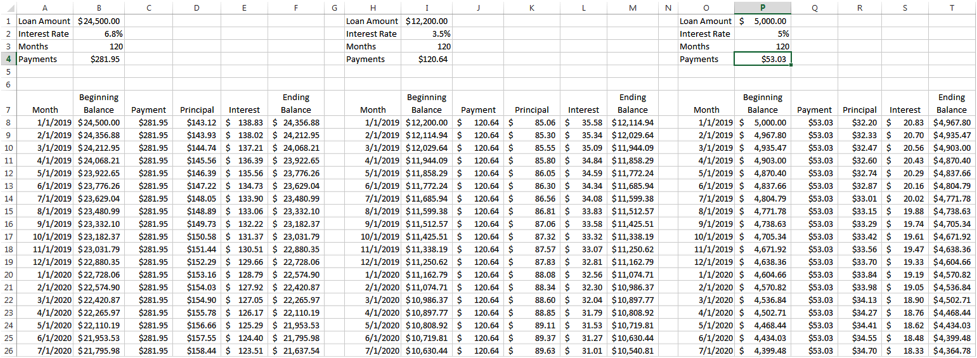
If you reviewed Part 1 of this series you should have an amortization schedule that looks something like this:

In my example, I used the standard ten year plan, so all three loans have 120 months’ worth of payments. Some things you can do with your table now that it’s completed is determine how much you will pay if you following the payment schedule. All you have to do is highlight the Excel cell below your last payment and hit the “AutoSum” button or “Ʃ” button. It should auto populate the correct cell range and create a formula that look like: =SUM(C8:C127). When I use this function, I get the following amounts

As you can see, under this repayment plan, I would pay $41,700 in principal and $12,974.48 in interest. If you were able to use an extended repayment plan and spread payments over 25 years, you would pay $36,405.97 in interest! However, your payment would drop from $455.62 to $260.36 per month. I chose the extended repayment plan on my $150,000 law school loans to both lower my payment and focus on payment off my highest interest rate first.
At this point, we are ready to add payments, increase payments, etc and see what effect they have on paying off the student loans quicker. Have you set a goal? If you remember, my goal was to pay off my loans in 7 years. Your goal may be to pay an additional $200 per month, or $2,500 twice a year when you get that extra paycheck, or a $10,000 lump sum payment at the end of each year. Either way, you will be able to manipulate your amortization table to find out what it will take to reach your goal.
For this example, let’s use a 7 year goal. The first step is to use a loan payment calculator to determine how much I’d have to pay monthly to reach that seven year goal. There are a number of financial calculators you can use, but I use BankRate’s loan calculator found here:
https://www.bankrate.com/calculators/mortgages/loan-calculator.aspx
It’s simple to use and quick. You enter in your balance, number of payments in month/years and your interest amount. Then Viola! You have your monthly payment. Starting with the $24,500 loan, I’ll enter 7 years and 6.8% interest, and I get a payment of $367.38. For the other two loans, I get payments of $163.97 and $70.67 for a total payment of $602.02. This is an increase of $146.40 per month over the ten year plan. Enter the three new monthly payment amounts in the payment column under the correct loan, i.e. C8 for the $24,500 loan. You can also add the excess by adding the additional amount into the formula: =$B$4+85.43. This option is useful if you want to add various payment amounts at different times. Once your new payment is entered, click on the lower right of the cell and drag all the way down to your projected payoff date. For a seven year payment, that would be 84th month and the 91st row in my table.

As you can see, by adding the interest paid in seven years for each loan, the total interest paid was $8,869.37 or a savings of $4,105.11 in interest over the ten year plan.
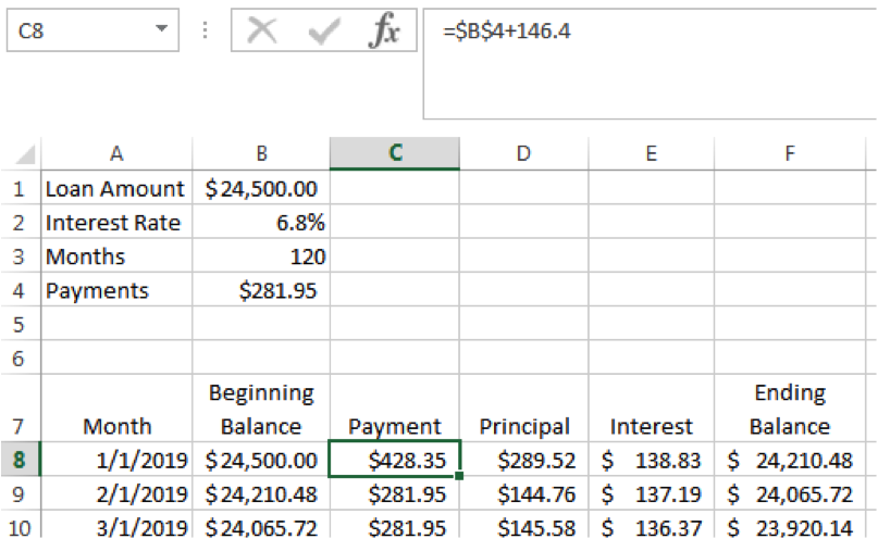
Now, let’s say you have that extra $146.40 per month, but you want to either follow the snowball plan (lower balance first) or the avalanche plan (highest interest first) in paying off your loans. For the avalanche plan I’m going to apply the full $146.40 per month to the $24,500 loan until I pay it off. To figure out how long this will take, I’ll insert “=$B$4+146.40” into the first payment cell and copy all the way down until I get to a “0” ending balance.

It will take almost six years to pay off this loan and will be paid off in month 70 with a final payment of $139.03:

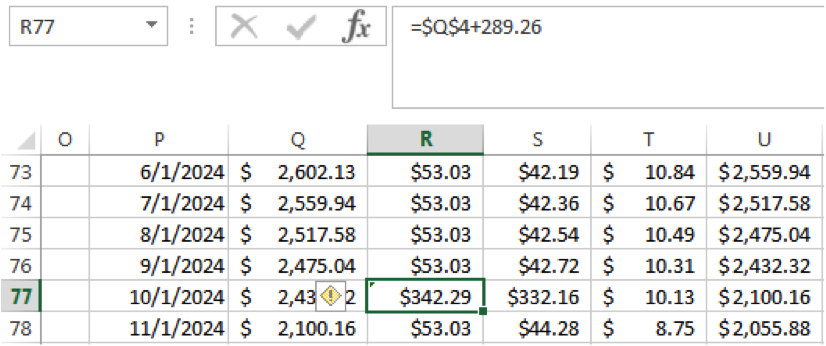
Next, you’re going to take the remainder of that payment $428.35 – $139.03 = $289.26 and add that to the payment of your next highest interest loan. In this case, it is the loan with the 5% interest rate (….or….you can always use this additional cash to celebrate paying off one of your loans. Just a thought).

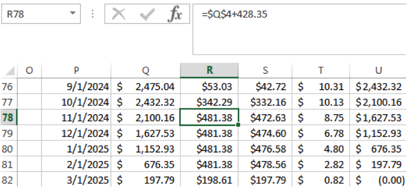
Then you’ll add the full payment of the loan you just paid off to the next payment. In this scenario, only four of these payments were need to be made to almost pay down this next loan. With a final payment of $198.79, the $5,000 loan was paid off in month 75.

Finally, we move those additional payment to the final loan, paying the full $602.02 until that loan is paid off completely. As you can see in the below, the loan is paid off in month 84 (right at the 7 year mark) but the payment is only $45.69 rather than the $602.02. My using the avalanche method, an additional $556.33 in interest was saved (You should definitely use that savings to celebrate paying off your loans!)

If you decide to use the snowball method, you’ll end up paying a little more in interest. In this example, using that method resulting in an extra month’s payment of $535.70, which is essentially the additional amount of interest paid.

So there you have it! How to use an amortization schedule to view different repayment plans and how additional payments can help you pay off your loans faster and with less interest. In my next post, I’ll reveal how I used this type of amortization table to develop my plan in paying off over $150,000 law school loans and an additional $17,000 in undergrad loans in seven years!


